A retiree with a solid plan - diversified portfolio, reasonable withdrawal rate, 90% Monte Carlo success rate - retires in January 2008. By March 2009, the portfolio is down 37%. Withdrawals continued through the crash. The plan that was supposed to last 30 years is now fighting for survival in year two.
This is not a hypothetical. It happened to millions of people. And the standard retirement calculator, running scenarios from a normal distribution, said this kind of crash was a once-in-14,000-years event.
Black swan events do not care about your model's opinion of their probability.
What Makes a Black Swan
Nassim Taleb defined three criteria: the event is rare, it has extreme impact, and after it happens, everyone explains why it was obvious. In financial markets, black swans are the crashes that standard models say should not happen - but do.
| Event | Year | Drawdown | "Should happen" under normal model |
|---|---|---|---|
| Black Monday | 1987 | -22% in one day | Once in 10^50 years |
| Dot-com bust | 2000-02 | -49% | Once in ~300 years |
| Global Financial Crisis | 2008 | -37% (single year) | Once in ~14,000 years |
| COVID crash | 2020 | -34% in 23 days | Once in ~10,000 years |
The common thread: each event was considered extremely unlikely by the prevailing models, and each happened within a single generation. The normal distribution is not slightly wrong about these events. It is wrong by orders of magnitude.
Why Retirees Are Uniquely Vulnerable
During your working years, a black swan is painful but survivable. You keep contributing, you buy at lower prices, and you have decades to recover. The math is different for a retiree who is withdrawing.
Consider the 2008 crash hitting in year 2 of a 30-year retirement. Starting portfolio: 1,000,000. Annual withdrawal: 40,000.
| Year | Start | Return | Withdrawal | End |
|---|---|---|---|---|
| 1 | 1,000,000 | +5% | 40,000 | 1,010,000 |
| 2 | 1,010,000 | -37% | 40,000 | 596,300 |
| 3 | 596,300 | +26% | 40,000 | 711,338 |
| 4 | 711,338 | +15% | 40,000 | 778,039 |
After two strong recovery years, the portfolio is still down 22% from where it started. The retiree withdrew 160,000 during this period - money that was not available to participate in the recovery. This is sequence-of-returns risk at its most destructive: a black swan event in the vulnerability window.
Now imagine the same crash hitting in year 25. The portfolio has had two decades of growth (even after withdrawals). A 37% drop from a 2,000,000 portfolio leaves 1,260,000 - still well above the starting balance. Same crash, same withdrawal rate, completely different outcome.
The timing of the black swan matters more than its magnitude. And timing is the one thing you cannot control.
How to Model Black Swans Properly
There are two complementary approaches, and a serious Monte Carlo retirement calculator should offer both.
Fat-tail distributions
Fat-tailed distributions like the Student's t replace the normal distribution's thin tails with heavier ones. Under a Student's t with 5 degrees of freedom, a 30%+ annual loss has a probability of about 3-4% - roughly once every 25-30 years. This matches the historical record far better than the normal distribution's "once per century" estimate.
Fat tails increase the frequency of extreme returns in both directions. They produce more crashes, but also more booms. The net effect on success rates is negative, because sequence-of-returns risk makes portfolios asymmetrically sensitive to crashes during withdrawal.
The advantage of fat tails is simplicity: you change one parameter (degrees of freedom) and the entire distribution adjusts. The downside is that the events are still random draws from a continuous distribution. They do not model the discrete, sudden nature of an actual crash.
Discrete black swan events
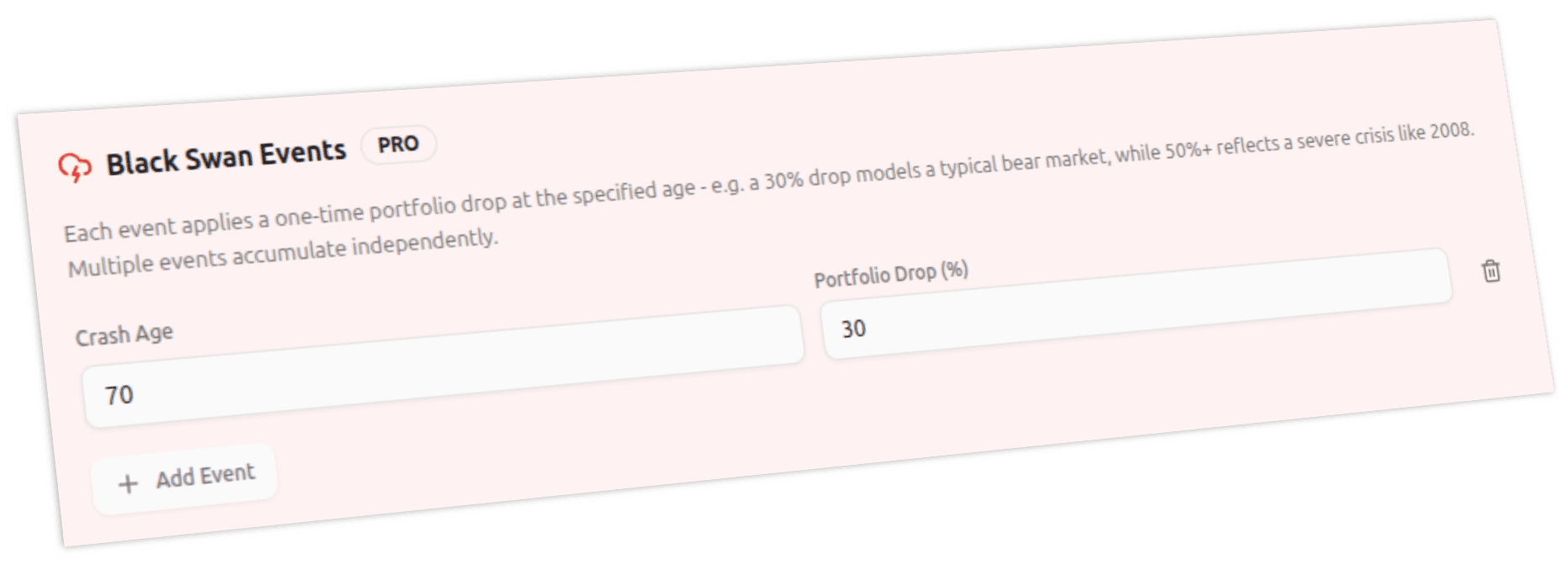
The second approach models black swans as a deliberate stress test: you pick a specific age at which a crash occurs and how severe it is. This is not a random event the simulator might or might not generate. It is a deterministic shock - "what happens if I lose 35% of my portfolio at age 67?"
You specify two things:
- Age: When does the crash hit? Testing age 66-70 (the first 5 years of a typical retirement) is the most revealing, since that is when sequence risk does the most damage.
- Drop percentage: How severe is the crash? A -35% drop mirrors 2008. A -50% drop tests a scenario worse than anything in modern history.
This approach layers a discrete crash on top of the normal (or fat-tailed) volatility in your simulation. Every iteration still has its own random return sequence, but all of them include the crash at the specified age. This tells you: "given that a crash of this magnitude happens at this point, how does my plan hold up across thousands of different recovery paths?"
The advantage is precision. Instead of wondering whether a random simulation happened to include a crash at the worst time, you force the worst timing and see the result. This is closer to how actual stress testing works in institutional risk management - test the specific scenario you are worried about, not just the average of all possibilities.
Combining Both Approaches
Fat tails and discrete shocks are not alternatives. They capture different aspects of tail risk.
Fat tails fix the baseline distribution: even "normal" bad years happen more often than a Gaussian model predicts. A -20% year is not rare - it happens roughly once a decade.
Discrete shocks let you stress-test a specific catastrophic scenario on top of that already-realistic baseline. You are not asking "what is the average outcome?" You are asking "what happens if the worst plausible crash lands at the worst plausible time?"
When you combine both, your Monte Carlo simulation produces:
- More frequent moderate crashes (from fat tails across all iterations)
- A guaranteed catastrophic crash at a specific age (from the discrete shock)
- Thousands of different recovery paths (each iteration has different returns before and after the shock)
The success rates you get from this combined model are typically 5-15 percentage points lower than a normal-distribution simulation. That gap is not pessimism. It is the risk your plan was hiding.
The First Five Years: Your Vulnerability Window
The interaction between black swans and sequence-of-returns risk creates a defined vulnerability window. Research consistently shows that portfolio outcomes are disproportionately determined by returns in the first 5-10 years of retirement.
A black swan in year 1-5 is devastating: the portfolio is at or near its starting value, withdrawals are at their maximum relative to the balance, and the recovery has to happen while money is still going out the door.
A black swan in year 15-20 is manageable: the portfolio has likely grown (despite withdrawals), the withdrawal rate relative to the current balance is lower, and there is still time for recovery.
This asymmetry has a practical implication: the first 5 years of retirement carry disproportionate risk, and black swan protection matters most during this window.
Strategies that help:
- Cash buffer (1-2 years of expenses): Avoid selling equities during the crash. Draw from cash instead and let the portfolio recover.
- Dynamic spending: Strategies like Guyton-Klinger guardrails automatically cut spending when the portfolio drops. A 10% spending cut during a crash dramatically improves recovery odds.
- Conservative initial allocation: A "bond tent" starts retirement with higher bond allocation (70/30 instead of 60/40) and gradually shifts toward equities over 5-10 years. This reduces the portfolio's exposure during the vulnerability window.
- Lower initial withdrawal rate: Starting at 3.5% instead of 4% provides a buffer that is invisible in good years but critical in bad ones. The 4% rule is already questionable under fat-tail assumptions; under black swan modeling, it becomes outright aggressive.
The Psychology of Black Swans
There is a behavioral dimension that models do not capture. When a black swan hits, retirees panic. They sell at the bottom, abandon their asset allocation, and lock in losses that the portfolio might have recovered from.
A Monte Carlo simulation assumes you follow the plan - that you keep withdrawing at the configured rate, you rebalance on schedule, and you do not sell everything and move to cash after a 30% drop. In reality, many retirees do exactly that, turning a temporary drawdown into a permanent loss.
This is another argument for building black swan scenarios into your planning process. If you have already seen what a 37% crash does to your plan - and you have seen that the plan survives with a spending cut and a two-year recovery - you are less likely to panic when it actually happens. The simulation is not just a planning tool. It is a psychological rehearsal.
What This Means for Your Plan
Test your plan against a specific crash at the worst timing. A fat-tailed model alone still relies on random chance to place a crash in your first few years. Force the scenario: set a -35% drop at age 66 and see if your plan survives across thousands of recovery paths.
Focus on the first 5 years. If your plan survives a black swan in year 2, it will likely survive one in year 15. Run the crash at different ages and see where the breaking point is. If early crashes break your plan, adjust your strategy for the vulnerability window.
Use flexible spending as your primary defense. The single most effective mitigation for black swan risk is the ability to cut spending temporarily. A 10-15% cut during a crash costs you a few years of slightly lower income. Failing to cut costs you the entire plan.
Remember that crashes are not rare. Historical data shows a drawdown of 30%+ roughly once every 25-30 years. Over a 30-year retirement, encountering at least one is more likely than not. It is not an edge case - it is a planning requirement.