A Monte Carlo retirement calculator runs thousands of simulated futures for your portfolio - each with a different sequence of market returns - and tells you the probability that your money lasts through retirement. Instead of a single "you'll have $X at age 85" answer, you get a distribution: best case, worst case, and everything in between.
That shift from a single number to a probability is what makes Monte Carlo fundamentally different from a spreadsheet projection.
How a Monte Carlo Retirement Calculator Works
The core idea is simple: randomize the unknown, repeat many times, and study the spread of results.
-
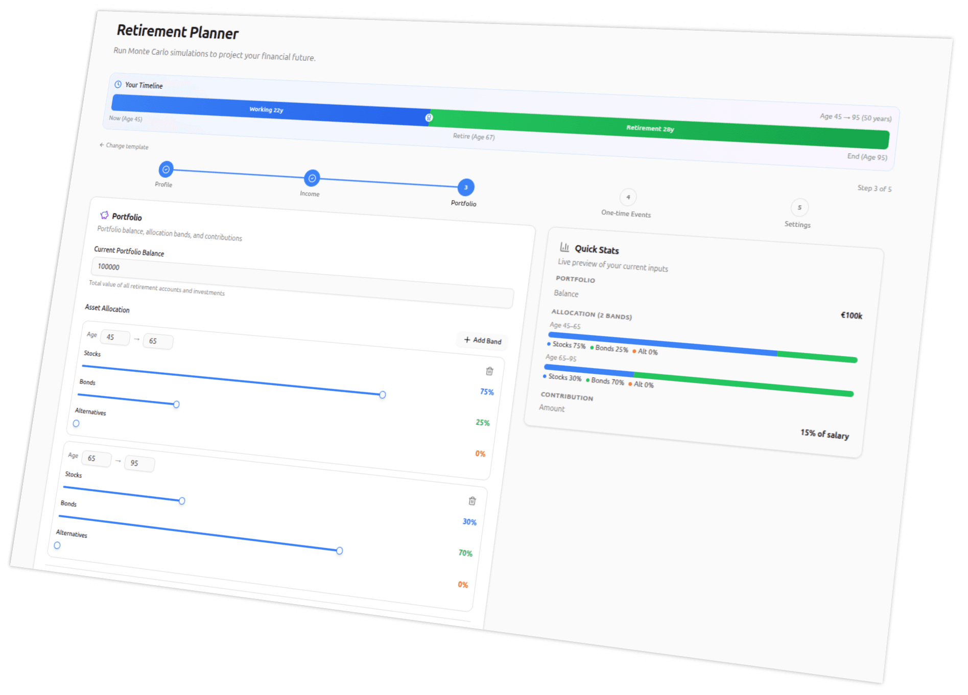
You define the inputs. Starting balance, asset allocation, expected returns and volatility for each asset class, withdrawal amount, and time horizon. These are the knowns - or at least your best estimates.
-
The calculator generates random returns. For each simulated year, it draws a return for each asset class from a probability distribution. In a basic calculator, that distribution is the normal (bell) curve. In a more advanced one, it might be a fat-tailed distribution like the Student's t - more on why that matters below.
-
It applies your spending plan. Subtract withdrawals, add any income (Social Security, pensions, part-time work), rebalance the portfolio, and move to the next year.
-
It repeats. A single run is one possible future. Run it 1,000 or 50,000 times, and you get a statistically meaningful sample of possible futures.
-
It aggregates the results. The key output is your success rate - the percentage of simulations where your money lasted the full horizon. You also get percentile bands showing the range of portfolio values over time.
Each iteration is not a prediction. No single run tells you what will happen. The power is in the aggregate - the shape of the distribution tells you how robust your plan really is.
Why a Fixed-Return Projection Falls Short
The alternative to Monte Carlo is the approach most simple retirement calculators use: assume a fixed annual return (say 7%), compound it forward, and report whether you run out of money.
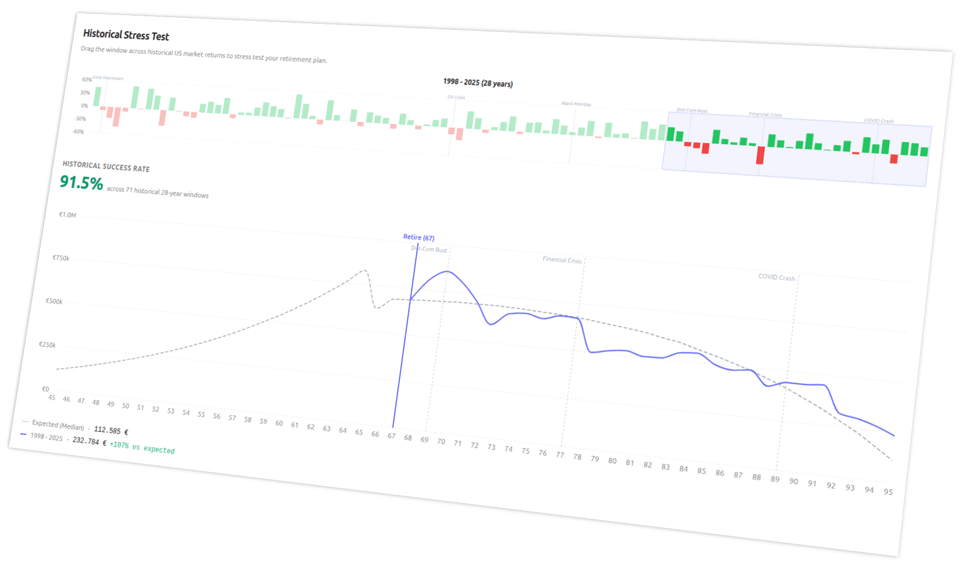
The problem is that this ignores volatility and sequence of returns. Two retirees who both earn an average of 7% over 30 years can have wildly different outcomes depending on when the good and bad years fall.
A retiree who hits a bear market in years 1-3 while withdrawing may deplete the portfolio decades earlier than one who hits the same bear market in years 25-27. The average return is identical. The outcome is not.
Monte Carlo captures this path dependency. A fixed-return projection cannot.
What Makes One Calculator Better Than Another
Not all Monte Carlo calculators are equal. The differences come down to a few key design choices:
Distribution choice
Most calculators assume returns follow a normal distribution - the classic bell curve. This is mathematically convenient but empirically wrong. Real market returns have fatter tails: extreme events (crashes and booms) happen more often than a bell curve predicts.
The 2008 financial crisis, for example, was roughly a 5-sigma event under Gaussian assumptions - something that should happen once every 14,000 years. It happened. So did 1987, 2000, and 2020.
A calculator that uses a Student's t-distribution or models black swan events as discrete shocks will give you a more honest picture of downside risk. If your retirement plan looks solid under normal assumptions, the real question is whether it survives the tails.
Iteration count
More iterations mean more stable estimates. At 100 iterations, your success rate might bounce around by several percentage points between runs. At 1,000, it stabilizes. At 10,000-50,000, the percentile bands converge and you can trust the numbers.
A calculator that only runs a few hundred iterations may give you a success rate that changes every time you click "run." That is noise, not signal. (We wrote more about how many iterations you actually need.)
Spending strategy flexibility
A fixed withdrawal amount is the simplest model, but real retirees adapt. Some cut spending in bad years (the Guyton-Klinger guardrail approach). Some spend a percentage of the remaining portfolio each year. Some set a floor and ceiling.
A calculator that only supports one strategy forces you to oversimplify. The strategy you choose can swing your success rate by 10-20 percentage points - it is not a minor detail.
Correlation modeling
Stocks, bonds, and alternative assets do not move independently. In a crisis, correlations spike - diversification benefits shrink exactly when you need them most. A calculator that models each asset as an independent coin flip overstates the benefit of diversification.
Cholesky-correlated returns model the relationship between asset classes, giving you a more realistic view of how your whole portfolio behaves under stress.

What Monte Carlo Cannot Do
Monte Carlo is powerful, but it is not a crystal ball. A few important caveats:
Garbage in, garbage out. If your return assumptions are wrong - say you assume 10% equity returns when the next decade delivers 4% - no amount of simulation will save the projection. Monte Carlo quantifies uncertainty within your assumptions, not the uncertainty of your assumptions. Choosing the right expected return for your simulation matters more than any other input. The same applies to country-specific calibration: the 4% rule was derived from US data and does not apply unmodified to European retirees.
It does not model regime changes. Most Monte Carlo models assume that the statistical properties of returns (mean, volatility, tail shape) are constant over the entire horizon. In reality, markets go through structurally different regimes. A 30-year horizon will span multiple regimes.
A success rate is not a guarantee. An 85% success rate means that in 15% of simulated scenarios, you ran out of money. Whether that risk is acceptable depends on your personal situation - how flexible your spending is, whether you have fallback income, and your tolerance for uncertainty. The headline number also hides important detail: see why a 90% success rate is not what you think for how to read the output beyond the summary metric.
The right way to use Monte Carlo is as a stress-testing tool, not a fortune-telling one. It answers "how would my plan hold up under a wide range of market conditions?" rather than "will my plan work?"
Frequently Asked Questions
- What is a good Monte Carlo success rate for retirement?
- Most planners target 80-95%. A 100% success rate usually means you are over-saving or under-spending. Below 75% means meaningful risk of running out. The right target depends on your spending flexibility - retirees who can cut back in bad years can comfortably accept lower success rates than those with rigid spending.
- How many iterations should a Monte Carlo retirement calculator run?
- At 500 iterations, results are noisy and shift several percentage points between runs. At 1,000-2,000, the success rate stabilizes for most plans. At 10,000-50,000, percentile bands and tail outcomes converge. Beyond 50,000, additional iterations yield diminishing returns.
- Is Monte Carlo simulation more accurate than historical backtesting?
- Neither is strictly more accurate - they answer different questions. Historical backtesting tells you how your plan would have performed in past market regimes. Monte Carlo generates synthetic scenarios that may include conditions history has not yet shown, like longer bear markets or bigger crashes.
- Why does my Monte Carlo result change every time I run it?
- Because Monte Carlo is a sampling method - each run draws different random returns. With under 1,000 iterations, the success rate can swing by several percentage points between runs. That is noise, not signal. A serious calculator runs enough iterations that successive runs produce nearly identical results.
- Can a Monte Carlo simulation predict a market crash?
- No. Monte Carlo does not predict anything - it stress-tests your plan across many possible futures. It can model how your portfolio would handle a crash if one occurs, but it does not forecast when or whether one will. Calculators that use fat-tailed distributions or black swan event modeling account for crashes more honestly than basic Gaussian models.